4.08 Quiz: Graph Polynomial Functions

four.4: Graphs of Polynomial Functions

Last updated
Save as PDF

Page ID: 29129

Learning Objectives

Recognize characteristics of graphs of polynomial functions.
Apply factoring to discover zeros of polynomial functions.
Identify zeros and their multiplicities.
Decide end behavior.
Understand the human relationship between degree and turning points.
Graph polynomial functions.
Apply the Intermediate Value Theorem.

The revenue in millions of dollars for a fictional cable company from 2006 through 2013 is shown in Table $\PageIndex{i}$.

Table $\PageIndex{i}$
Twelvemonth	2006	2007	2008	2009	2010	2011	2012	2013
Revenues	52.4	52.8	51.ii	49.five	48.6	48.6	48.7	47.1

The revenue tin be modeled by the polynomial part

\[R(t)=−0.037t^four+one.414t^three−19.777t^2+118.696t−205.332\]

where $R$ represents the revenue in millions of dollars and $t$ represents the twelvemonth, with $t=6$ corresponding to 2006. Over which intervals is the revenue for the company increasing? Over which intervals is the acquirement for the company decreasing? These questions, along with many others, tin exist answered by examining the graph of the polynomial function. We have already explored the local behavior of quadratics, a special case of polynomials. In this department we will explore the local beliefs of polynomials in general.

Recognizing Characteristics of Graphs of Polynomial Functions

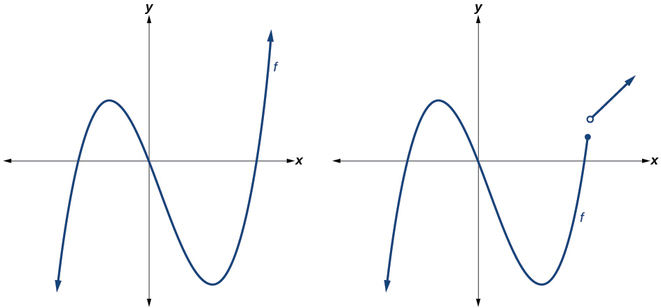
Polynomial functions of caste 2 or more have graphs that do non have sharp corners; retrieve that these types of graphs are called smooth curves. Polynomial functions as well brandish graphs that have no breaks. Curves with no breaks are called continuous. Figure $\PageIndex{one}$ shows a graph that represents a polynomial office and a graph that represents a function that is not a polynomial.

Graph of f(x)=x^3-0.01x — Figure $\PageIndex{ane}$: Graph of $f(ten)=x^three-0.01x$.

Example $\PageIndex{1}$: Recognizing Polynomial Functions

Which of the graphs in Figure $\PageIndex{two}$ represents a polynomial function?

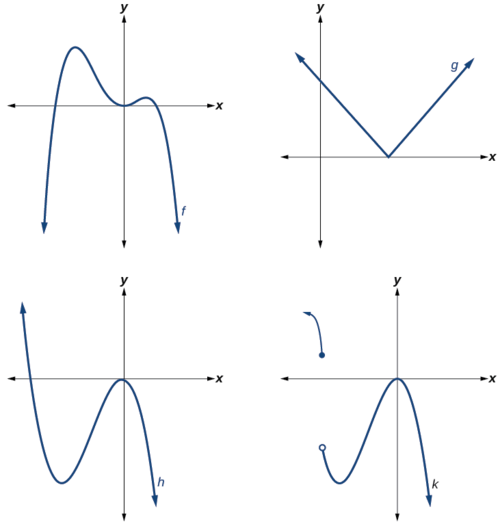
$Two graphs in which one has a polynomial function and the other has a function closely resembling a polynomial but is not. Two graphs in which one has a polynomial function and the other has a function closely resembling a polynomial but is not.$
Figure $\PageIndex{2}$

Solution

The graphs of $f$ and $h$ are graphs of polynomial functions. They are polish and continuous.
The graphs of $yard$ and $k$ are graphs of functions that are not polynomials. The graph of role $g$ has a abrupt corner. The graph of function $thousand$ is not continuous.

Q&A

Practise all polynomial functions have as their domain all real numbers?

Yes. Any real number is a valid input for a polynomial function.

Using Factoring to Find Zeros of Polynomial Functions

Call up that if $f$ is a polynomial function, the values of $x$ for which $f(ten)=0$ are called zeros of $f$. If the equation of the polynomial function can exist factored, nosotros can set each factor equal to zero and solve for the zeros.

We can use this method to observe x-intercepts because at the 10-intercepts we find the input values when the output value is zero. For general polynomials, this can be a challenging prospect. While quadratics tin can exist solved using the relatively simple quadratic formula, the corresponding formulas for cubic and quaternary-degree polynomials are not elementary enough to remember, and formulas exercise not exist for full general higher-degree polynomials. Consequently, we will limit ourselves to three cases in this department:

The polynomial can be factored using known methods: greatest common factor and trinomial factoring.
The polynomial is given in factored class.
Technology is used to determine the intercepts.

HOwTO: Given a polynomial role $f$, find the x-intercepts by factoring

Set $f(x)=0$.
If the polynomial function is not given in factored form:
1. Cistron out any common monomial factors.
2. Gene any factorable binomials or trinomials.
Set each factor equal to zero and solve to discover the x-intercepts.

Example $\PageIndex{ii}$: Finding the x-Intercepts of a Polynomial Function by Factoring

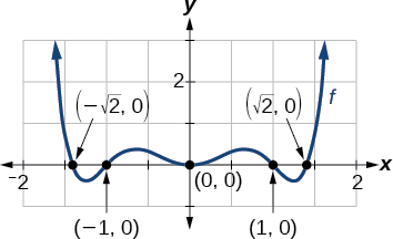
Find the ten-intercepts of $f(x)=x^6−3x^four+2x^2$.

Solution

We can attempt to factor this polynomial to discover solutions for $f(x)=0$.

\[\begin{marshal*} x^6−3x^4+2x^two&=0 & &\text{Factor out the greatest mutual cistron.} \\ x^2(x^iv−3x^two+2)&=0 & &\text{Factor the trinomial.} \\ x^2(x^2−ane)(10^2−2)&=0 & &\text{Set each factor equal to zero.} \end{align*}\]

\[\begin{align*} x^two&=0 & & & (10^2−i)&=0 & & & (10^ii−2)&=0 \\ x^2&=0 & &\text{ or } & x^2&=one & &\text{ or } & x^2&=2 \\ x&=0 &&& 10&={\pm}1 &&& x&={\pm}\sqrt{2} \finish{align*}\] .

This gives u.s.a. 5 x-intercepts: $(0,0)$, $(one,0)$, $(−1,0)$, $(\sqrt{two},0)$,and $(−\sqrt{2},0)$ (Figure $\PageIndex{3}$). We can see that this is an fifty-fifty function.

An even function — Figure $\PageIndex{3}$.

Example $\PageIndex{3}$: Finding the ten-Intercepts of a Polynomial Function by Factoring

Detect the x-intercepts of $f(ten)=10^3−5x^two−ten+v$.

Solution

Find solutions for $f(x)=0$ by factoring.

\[\brainstorm{align*} x^three−5x^two−x+five&=0 &\text{Factor by grouping.} \\ x^2(ten−five)−(x−five)&=0 &\text{Factor out the common factor.} \\ (ten^2−i)(ten−5)&=0 &\text{Factor the difference of squares.} \\ (x+i)(x−ane)(x−five)&=0 &\text{Set up each cistron equal to naught.} \end{align*}\]

\[\begin{align*} ten+ane&=0 & &\text{or} & x−one&=0 & &\text{or} & 10−5&=0 \\ x&=−one &&& x&=one &&& x&=5\end{align*}\]

At that place are iii x-intercepts: $(−1,0)$, $(1,0)$, and $(5,0)$ (Figure $\PageIndex{4}$).

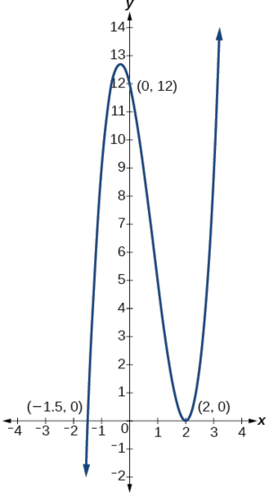
Graph of f(x)=x^3-5x^2-x+5 with its three intercepts (-1, 0), (1, 0), and (5, 0). — Effigy $\PageIndex{4}$: Graph of $f(x)$.

Example $\PageIndex{4}$: Finding the y- and x-Intercepts of a Polynomial in Factored Form

Discover the y- and x-intercepts of $yard(ten)=(x−ii)^2(2x+3)$.

Solution

The y-intercept tin can be plant by evaluating $g(0)$.

\[\begin{align*} g(0)&=(0−2)^2(2(0)+iii) \\ &=12 \terminate{align*}\]

So the y-intercept is $(0,12)$.

The 10-intercepts can be found past solving $grand(x)=0$.

\[(x−two)^2(2x+iii)=0\]

\[\begin{align*} (x−2)^ii&=0 & & & (2x+iii)&=0 \\ x−2&=0 & &\text{or} & x&=−\dfrac{three}{two} \\ 10&=2 \terminate{align*}\]

So the x-intercepts are $(2,0)$ and $\left(−\dfrac{3}{2},0\correct)$.

Analysis

We can e'er bank check that our answers are reasonable by using a graphing calculator to graph the polynomial as shown in Figure $\PageIndex{5}$.

Graph of g(x)=(x-2)^2(2x+3) with its two x-intercepts (2, 0) and (-3/2, 0) and its y-intercept (0, 12). — Figure $\PageIndex{5}$: Graph of $g(x)$.

Instance $\PageIndex{5}$: Finding the 10-Intercepts of a Polynomial Office Using a Graph

Detect the x-intercepts of $h(10)=x^3+4x^2+x−vi$.

Solution

This polynomial is not in factored form, has no common factors, and does non appear to be factorable using techniques previously discussed. Fortunately, we tin can use engineering science to discover the intercepts. Keep in mind that some values brand graphing difficult by mitt. In these cases, we tin have advantage of graphing utilities.

Looking at the graph of this function, as shown in Figure $\PageIndex{6}$, it appears that there are 10-intercepts at $x=−3,−2, \text{ and }1$.

Graph of h(x)=x^3+4x^2+x-6. — Figure $\PageIndex{half dozen}$: Graph of $h(x)$.

We can check whether these are correct by substituting these values for $x$ and verifying that
\[h(−three)=h(−2)=h(i)=0. \nonumber\]

Since $h(x)=x^3+4x^2+10−vi$, nosotros have:

\[ \begin{align*} h(−iii)&=(−3)^three+4(−iii)^2+(−3)−six=−27+36−3−6=0 \\[4pt] h(−two) &=(−2)^3+iv(−two)^two+(−2)−6 =−8+16−two−6=0 \\[4pt] h(ane)&=(1)^3+4(1)^2+(i)−6=ane+4+1−vi=0 \end{align*}\]

Each ten-intercept corresponds to a null of the polynomial function and each zero yields a gene, so we tin can now write the polynomial in factored class.

\[\begin{align*} h(x)&=x^three+4x^2+x−6 \\ &=(x+3)(x+2)(ten−1) \end{align*}\]

Do $\PageIndex{1}$

Find the y-and ten-intercepts of the office $f(x)=ten^iv−19x^2+30x$.

Answer

y-intercept $(0,0)$;
x-intercepts $(0,0)$, $(–v,0)$, $(2,0)$, and $(three,0)$

Identifying Zeros and Their Multiplicities

Graphs acquit differently at various x-intercepts. Sometimes, the graph will cross over the horizontal centrality at an intercept. Other times, the graph volition touch the horizontal axis and bounce off. Suppose, for example, we graph the function

\[f(ten)=(x+three)(x−2)^ii(x+one)^3.\]

Notice in Figure $\PageIndex{7}$ that the behavior of the function at each of the x-intercepts is unlike.

Graph of f(x)=(x+3)(x-2)^2(x+1)^3. — Effigy $\PageIndex{7}$: Identifying the behavior of the graph at an x-intercept past examining the multiplicity of the zero.

The x-intercept −3 is the solution of equation $(ten+3)=0$. The graph passes directly through thex-intercept at $ten=−3$. The factor is linear (has a degree of 1), and so the behavior nigh the intercept is like that of a line—it passes directly through the intercept. We call this a single zero because the zippo corresponds to a unmarried factor of the part.

The 10-intercept ii is the repeated solution of equation $(x−2)^2=0$. The graph touches the axis at the intercept and changes management. The factor is quadratic (degree 2), so the behavior virtually the intercept is like that of a quadratic—information technology bounces off of the horizontal axis at the intercept.

\[(x−ii)^two=(x−2)(x−2)\]

The factor is repeated, that is, the factor $(10−2)$ appears twice. The number of times a given factor appears in the factored form of the equation of a polynomial is called the multiplicity. The nix associated with this factor, $ten=2$, has multiplicity 2 because the factor $(x−2)$ occurs twice.

The x-intercept −i is the repeated solution of factor $(x+1)^3=0$.The graph passes through the axis at the intercept, merely flattens out a flake first. This factor is cubic (caste 3), then the behavior virtually the intercept is like that of a cubic—with the same S-shape most the intercept as the toolkit function $f(x)=ten^3$. We call this a triple nil, or a nil with multiplicity three.

For zeros with even multiplicities, the graphs bear on or are tangent to the x-axis. For zeros with odd multiplicities, the graphs cantankerous or intersect the x-axis. Come across Figure $\PageIndex{viii}$ for examples of graphs of polynomial functions with multiplicity 1, 2, and 3.

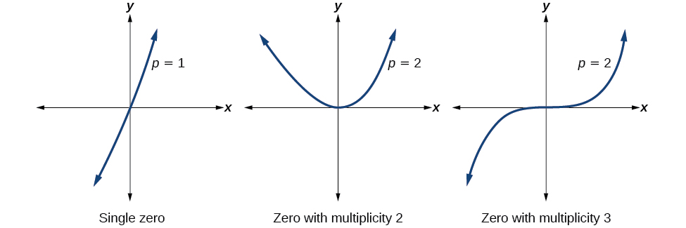
Three graphs showing three different polynomial functions with multiplicity 1, 2, and 3. — Figure $\PageIndex{viii}$: Three graphs showing iii dissimilar polynomial functions with multiplicity 1, 2, and three.

For college even powers, such every bit 4, 6, and 8, the graph will yet touch and bounce off of the horizontal axis but, for each increasing even power, the graph will appear flatter equally it approaches and leaves the x-axis.

For higher odd powers, such as v, 7, and 9, the graph will still cross through the horizontal axis, but for each increasing odd power, the graph will announced flatter as it approaches and leaves the x-axis.

Graphical Behavior of Polynomials at x-Intercepts

If a polynomial contains a factor of the form $(x−h)^p$, the behavior nigh the x-intercepth is determined past the power $p$. We say that $x=h$ is a goose egg of multiplicity $p$.

The graph of a polynomial function will bear upon the x-centrality at zeros with even multiplicities. The graph will cross the x-centrality at zeros with odd multiplicities.

The sum of the multiplicities is the degree of the polynomial function.

HOWTO: Given a graph of a polynomial function of degree $northward$, identify the zeros and their multiplicities

If the graph crosses the x-axis and appears nearly linear at the intercept, it is a unmarried goose egg.
If the graph touches the 10-axis and bounces off of the axis, it is a zero with fifty-fifty multiplicity.
If the graph crosses the 10-axis at a nix, information technology is a zero with odd multiplicity.
The sum of the multiplicities is $northward$.

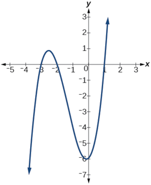
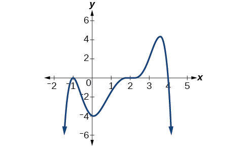
Example $\PageIndex{6}$: Identifying Zeros and Their Multiplicities

Use the graph of the function of caste half dozen in Figure $\PageIndex{9}$ to place the zeros of the role and their possible multiplicities.

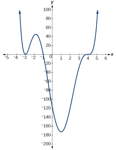
Graph of an even-degree polynomial with degree 6. — Figure $\PageIndex{9}$: Graph of a polynomial function with degree v.

Solution

The polynomial role is of degree $due north$. The sum of the multiplicities must be $n$.

Starting from the left, the first zero occurs at $ten=−3$. The graph touches the ten-axis, so the multiplicity of the zero must be even. The nil of −three has multiplicity 2.

The adjacent goose egg occurs at $x=−one$. The graph looks nearly linear at this point. This is a single nothing of multiplicity 1.

The last cipher occurs at $x=four$.The graph crosses the 10-axis, so the multiplicity of the zero must be odd. We know that the multiplicity is likely 3 and that the sum of the multiplicities is probable 6.

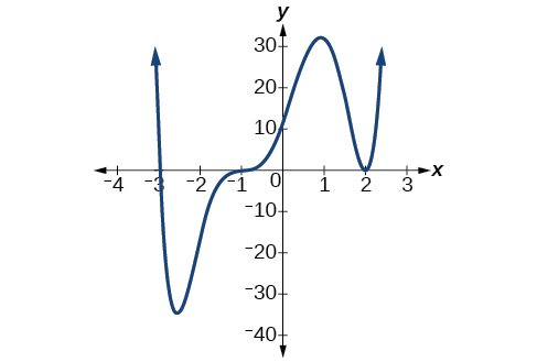
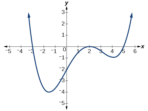
Exercise $\PageIndex{2}$

Employ the graph of the function of caste 5 in Figure $\PageIndex{10}$ to identify the zeros of the function and their multiplicities.

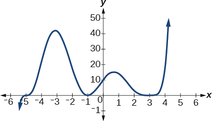
$Graph of a polynomial function with degree 5.$

Figure $\PageIndex{10}$: Graph of a polynomial function with degree 5.

Reply: The graph has a zip of –5 with multiplicity one, a null of –1 with multiplicity 2, and a cipher of three with even multiplicity.

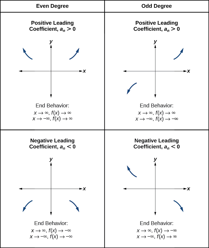
Determining End Behavior

As we have already learned, the behavior of a graph of a polynomial function of the form

\[f(x)=a_nx^n+a_{n−1}x^{n−ane}+...+a_1x+a_0\]

will either ultimately rise or autumn as $10$ increases without bound and will either rising or fall every bit $x$ decreases without bound. This is because for very big inputs, say 100 or one,000, the leading term dominates the size of the output. The same is true for very small inputs, say –100 or –1,000.

Think that we call this beliefs the terminate behavior of a function. As nosotros pointed out when discussing quadratic equations, when the leading term of a polynomial function, $a_nx^north$, is an even power function, as $x$ increases or decreases without bound, $f(x)$ increases without bound. When the leading term is an odd power function, every bit $x$ decreases without bound, $f(10)$ as well decreases without spring; equally $x$ increases without bound, $f(x)$ as well increases without bound. If the leading term is negative, it will change the direction of the end beliefs. Figure $\PageIndex{xi}$ summarizes all 4 cases.

Table showing the end behavior of odd and even polynomials with positive and negative coefficients — Effigy $\PageIndex{11}$.

Agreement the Human relationship betwixt Caste and Turning Points

In addition to the end behavior, recall that we can analyze a polynomial function's local beliefs. It may accept a turning point where the graph changes from increasing to decreasing (rising to falling) or decreasing to increasing (falling to rising). Look at the graph of the polynomial function $f(x)=x^iv−x^3−4x^two+4x$ in Figure $\PageIndex{12}$. The graph has three turning points.

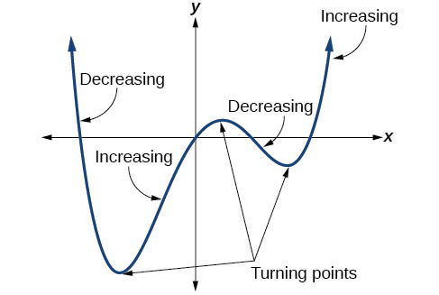
Graph of f(x)=x^4-x^3-4x^2+4x which denotes where the function increases and decreases and its turning points. — Figure $\PageIndex{12}$: Graph of $f(x)=10^four-ten^iii-4x^2+4x$

This role $f$ is a quaternary degree polynomial office and has three turning points. The maximum number of turning points of a polynomial function is e'er one less than the caste of the function.

Definition: Interpreting Turning Points

A turning bespeak is a point of the graph where the graph changes from increasing to decreasing (rising to falling) or decreasing to increasing (falling to ascension). A polynomial of degree $n$ will have at virtually $n−1$ turning points.

Example $\PageIndex{7}$: Finding the Maximum Number of Turning Points Using the Degree of a Polynomial Function

Find the maximum number of turning points of each polynomial part.

$f(x)=−x^3+4x^five−3x^2+1$
$f(x)=−(x−ane)^2(1+2x^two)$

Solution

a. $f(ten)=−x^3+4x^5−3x^two+1$

First, rewrite the polynomial part in descending order: $f(x)=4x^5−10^three−3x^2+one$

Identify the degree of the polynomial function. This polynomial office is of caste five.

The maximum number of turning points is $5−ane=4$.

b. $f(x)=−(x−1)^2(1+2x^2)$

First, identify the leading term of the polynomial function if the part were expanded.

$imageedit_33_3540887475.png$

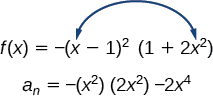
And then, identify the degree of the polynomial role. This polynomial function is of caste 4.

The maximum number of turning points is $4−1=three$.

Graphing Polynomial Functions

We can use what we accept learned about multiplicities, end beliefs, and turning points to sketch graphs of polynomial functions. Let united states of america put this all together and expect at the steps required to graph polynomial functions.

Howto: Given a polynomial part, sketch the graph

Find the intercepts.
Check for symmetry. If the function is an even function, its graph is symmetrical nearly the y-centrality, that is, $f(−x)=f(x)$. If a function is an odd function, its graph is symmetrical about the origin, that is, $f(−x)=−f(x)$.
Use the multiplicities of the zeros to determine the behavior of the polynomial at the x-intercepts.
Determine the cease behavior by examining the leading term.
Use the terminate beliefs and the beliefs at the intercepts to sketch a graph.
Ensure that the number of turning points does not exceed i less than the caste of the polynomial.
Optionally, apply technology to check the graph.

Example $\PageIndex{8}$: Sketching the Graph of a Polynomial Office

Sketch a graph of $f(10)=−2(10+3)^2(x−v)$.

Solution

This graph has two 10-intercepts. At $ten=−3$, the factor is squared, indicating a multiplicity of two. The graph volition bounce at this x-intercept. At $x=5$,the function has a multiplicity of i, indicating the graph volition cross through the axis at this intercept.

The y-intercept is institute by evaluating $f(0)$.

\[\begin{align*} f(0)&=−2(0+3)^2(0−v) \\ &=−2⋅9⋅(−5) \\ &=90 \end{align*}\]

The y-intercept is $(0,xc)$.

Additionally, we can see the leading term, if this polynomial were multiplied out, would be $−2x3$, so the end behavior is that of a vertically reflected cubic, with the outputs decreasing as the inputs approach infinity, and the outputs increasing every bit the inputs approach negative infinity. See Effigy $\PageIndex{xiii}$.

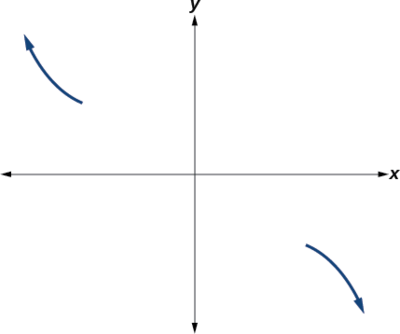
Figure $\PageIndex{xiii}$: Showing the distribution for the leading term.

To sketch this, we consider that:

As $x{\rightarrow}−{\infty}$ the function $f(10){\rightarrow}{\infty}$,and so nosotros know the graph starts in the second quadrant and is decreasing toward the ten-axis.
Since $f(−ten)=−two(−x+3)^2(−x–5)$ is not equal to $f(x)$, the graph does non display symmetry.
At $(−iii,0)$, the graph bounces off of thex-centrality, and then the part must start increasing.
At $(0,90)$, the graph crosses the y-axis at the y-intercept. See Figure $\PageIndex{xiv}$.

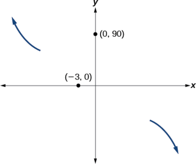
Graph of the end behavior and intercepts, (-3, 0) and (0, 90), for the function f(x)=-2(x+3)^2(x-5). — Effigy $\PageIndex{14}$: Graph of the stop behavior and intercepts, $(-3, 0)$ and $(0, ninety)$, for the function $f(x)=-2(ten+iii)^2(ten-5)$.

Somewhere after this point, the graph must turn back down or start decreasing toward the horizontal centrality because the graph passes through the next intercept at $(5,0)$. See Effigy $\PageIndex{xv}$.

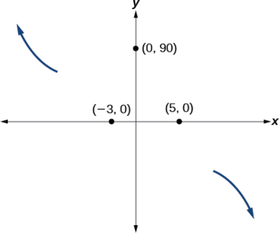
Graph of the end behavior and intercepts, (-3, 0), (0, 90) and (5, 0), for the function f(x)=-2(x+3)^2(x-5). — Figure $\PageIndex{15}$: Graph of the end behavior and intercepts, $(-3, 0)$, $(0, ninety)$ and $(5, 0)$, for the function $f(x)=-2(10+three)^2(x-5)$.

As $x{\rightarrow}{\infty}$ the function $f(10){\rightarrow}−{\infty}$,

so we know the graph continues to decrease, and nosotros can stop drawing the graph in the fourth quadrant.

Using technology, we can create the graph for the polynomial function, shown in Effigy $\PageIndex{sixteen}$, and verify that the resulting graph looks like our sketch in Figure $\PageIndex{15}$.

$The complete graph of the polynomial function f(x)=−2(x+3)^2(x−5)$
Effigy $\PageIndex{xvi}$: The complete graph of the polynomial part $f(ten)=−2(x+three)^2(x−v)$.

Practice $\PageIndex{8}$

Sketch a graph of $f(x)=\dfrac{1}{iv}x(10−one)^four(ten+3)^3$.

Answer: $alt$
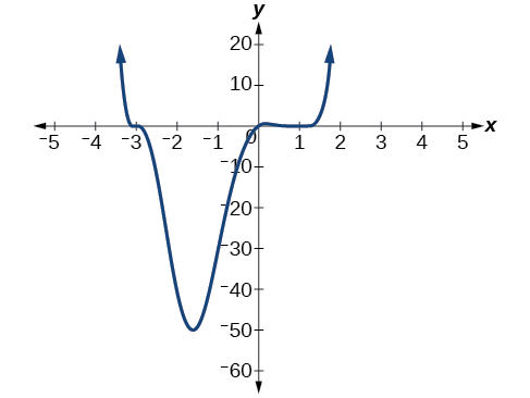
Figure $\PageIndex{17}$: Graph of $f(ten)=\frac{1}{4}x(x−1)^four(x+three)^3$

In some situations, nosotros may know two points on a graph just not the zeros. If those 2 points are on contrary sides of the ten-axis, nosotros tin confirm that there is a aught between them. Consider a polynomial function $f$ whose graph is smooth and continuous. The Intermediate Value Theorem states that for two numbers $a$ and $b$ in the domain of $f$,if $a<b$ and $f(a){\neq}f(b)$,and so the function $f$ takes on every value between $f(a)$ and $f(b)$. We tin apply this theorem to a special case that is useful in graphing polynomial functions. If a point on the graph of a continuous function $f$ at $10=a$ lies in a higher place the x-axis and another indicate at $10=b$ lies below thex-axis, there must exist a third point between $x=a$ and $x=b$ where the graph crosses the x-centrality. Call this point $(c,f(c))$.This means that nosotros are assured there is a solution $c$ where $f(c)=0$.

In other words, the Intermediate Value Theorem tells us that when a polynomial office changes from a negative value to a positive value, the office must cross the x-axis. Effigy $\PageIndex{18}$ shows that at that place is a nix between $a$ and $b$.

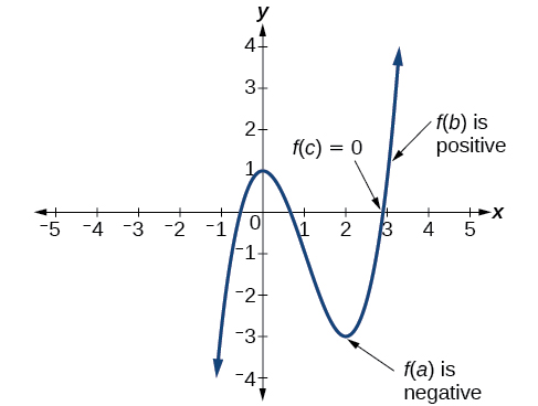
Graph of an odd-degree polynomial function that shows a point f(a) that's negative, f(b) that's positive, and f(c) that's 0. — Figure $\PageIndex{eighteen}$: Using the Intermediate Value Theorem to bear witness there exists a goose egg.

Definition: Intermediate Value Theorem

Let $f$ be a polynomial function. The Intermediate Value Theorem states that if $f(a)$ and $f(b)$ accept opposite signs, then there exists at least i value $c$ between $a$ and $b$ for which $f(c)=0$.

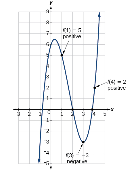
Example $\PageIndex{9}$: Using the Intermediate Value Theorem

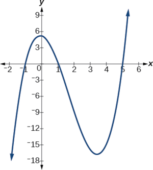
Prove that the function $f(x)=ten^3−5x^two+3x+6$ has at least two real zeros between $x=1$ and $x=4$.

Solution

As a start, evaluate $f(10)$ at the integer values $x=i,\;ii,\;three,\; \text{and }4$ (Table $\PageIndex{2}$).

Table $\PageIndex{2}$
$10$	1	two	3	4
$f(x)$	5	0	-3	2

Nosotros see that i zero occurs at $10=two$. As well, since $f(three)$ is negative and $f(4)$ is positive, by the Intermediate Value Theorem, there must be at to the lowest degree one real zero between 3 and four.

We take shown that there are at least two real zeros between $x=i$ and $x=4$.

Analysis

We tin can besides come across on the graph of the function in Effigy $\PageIndex{xix}$ that in that location are two real zeros between $x=1$ and $x=4$.

Graph of f(x)=x^3-5x^2+3x+6 and shows, by the Intermediate Value Theorem, that there exists two zeros since f(1)=5 and f(4)=2 are positive and f(3) = -3 is negative. — Figure $\PageIndex{19}$.

Exercise $\PageIndex{4}$

Testify that the office $f(x)=7x^5−9x^iv−10^2$ has at least one real zippo between $x=1$ and $ten=2$.

Answer: Considering $f$ is a polynomial function and since $f(1)$ is negative and $f(2)$ is positive, there is at to the lowest degree i existent goose egg between $x=1$ and $x=2$.

Writing Formulas for Polynomial Functions

Now that we know how to find zeros of polynomial functions, we can use them to write formulas based on graphs. Because a polynomial function written in factored form will have an x-intercept where each cistron is equal to zero, nosotros can course a function that will laissez passer through a set up of x-intercepts by introducing a corresponding set of factors.

Note: Factored Form of Polynomials

If a polynomial of everyman degree $p$ has horizontal intercepts at $ten=x_1,x_2,…,x_n$, then the polynomial can be written in the factored class: $f(10)=a(x−x_1)^{p_1}(10−x_2)^{p_2}⋯(ten−x_n)^{p_n}$ where the powers $p_i$ on each factor can exist determined by the beliefs of the graph at the corresponding intercept, and the stretch factor $a$ can be determined given a value of the role other than the x-intercept.

$alt$ Given a graph of a polynomial function, write a formula for the function.

Identify the x-intercepts of the graph to find the factors of the polynomial.
Examine the behavior of the graph at the ten-intercepts to determine the multiplicity of each factor.
Find the polynomial of least degree containing all the factors found in the previous step.
Use whatever other point on the graph (the y-intercept may be easiest) to determine the stretch factor.

Instance $\PageIndex{x}$: Writing a Formula for a Polynomial Role from the Graph

Write a formula for the polynomial function shown in Figure $\PageIndex{20}$.

Graph of a positive even-degree polynomial with zeros at x=-3, 2, 5 and y=-2. — Effigy $\PageIndex{twenty}$.

Solution

This graph has three x-intercepts: $x=−iii,\;2,\text{ and }five$. The y-intercept is located at $(0,2)$.At $x=−three$ and $ ten=5$, the graph passes through the axis linearly, suggesting the respective factors of the polynomial will be linear. At $x=ii$, the graph bounces at the intercept, suggesting the respective factor of the polynomial will be 2nd degree (quadratic). Together, this gives us

\[f(x)=a(ten+3)(x−2)^2(x−5)\]

To determine the stretch gene, nosotros employ another indicate on the graph. We volition use the y-intercept $(0,–2)$, to solve for $a$.

\[\brainstorm{marshal*} f(0)&=a(0+3)(0−2)^2(0−5) \\ −2&=a(0+three)(0−ii)^2(0−5) \\ −2&=−60a \\ a&=\dfrac{1}{30} \finish{align*}\]

The graphed polynomial appears to represent the function $f(x)=\dfrac{ane}{30}(x+3)(10−2)^two(x−five)$.

Exercise $\PageIndex{v}$

Given the graph shown in Figure $\PageIndex{21}$, write a formula for the role shown.

Graph of a negative even-degree polynomial with zeros at x=-1, 2, 4 and y=-4. — Effigy $\PageIndex{21}$.

Answer: $f(x)=−\frac{1}{viii}(ten−ii)^3(x+1)^2(x−four)$

Using Local and Global Extrema

With quadratics, we were able to algebraically observe the maximum or minimum value of the function by finding the vertex. For general polynomials, finding these turning points is not possible without more advanced techniques from calculus. Even so, finding where extrema occur tin still exist algebraically challenging. For now, nosotros will estimate the locations of turning points using technology to generate a graph.

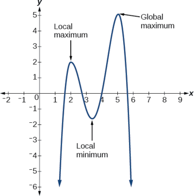
Each turning signal represents a local minimum or maximum. Sometimes, a turning point is the highest or lowest point on the unabridged graph. In these cases, we say that the turning signal is a global maximum or a global minimum. These are also referred to as the absolute maximum and absolute minimum values of the part.

Note: Local and Global Extrema

A local maximum or local minimum at $x=a$ (sometimes called the relative maximum or minimum, respectively) is the output at the highest or lowest signal on the graph in an open interval effectually $x=a$.If a role has a local maximum at $a$, then $f(a){\geq}f(x)$for all $x$ in an open up interval effectually $x=a$. If a function has a local minimum at $a$, and then $f(a){\leq}f(x)$for all $x$ in an open interval around $10=a$.

A global maximum or global minimum is the output at the highest or lowest point of the function. If a part has a global maximum at $a$, then $f(a){\geq}f(x)$ for all $x$. If a office has a global minimum at $a$, and then $f(a){\leq}f(x)$ for all $x$.

Nosotros can see the difference between local and global extrema in Effigy $\PageIndex{22}$.

Graph of an even-degree polynomial that denotes the local maximum and minimum and the global maximum. — Figure $\PageIndex{22}$: Graph of an even-caste polynomial that denotes the local maximum and minimum and the global maximum.

$alt$ Practise all polynomial functions have a global minimum or maximum?

No. Merely polynomial functions of fifty-fifty caste accept a global minimum or maximum. For example, $f(x)=x$ has neither a global maximum nor a global minimum.

Example $\PageIndex{xi}$: Using Local Extrema to Solve Applications

An open-peak box is to be constructed by cutting out squares from each corner of a 14 cm by 20 cm sail of plastic so folding up the sides. Find the size of squares that should exist cut out to maximize the book enclosed by the box.

Solution

We will start this problem by cartoon a picture like that in Figure $\PageIndex{23}$, labeling the width of the cut-out squares with a variable, $w$.

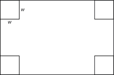
Diagram of a rectangle with four squares at the corners. — Figure $\PageIndex{23}$: Diagram of a rectangle with iv squares at the corners.

Notice that after a square is cut out from each end, it leaves $a(14−2w)$ cm past $(20−2w)$ cm rectangle for the base of the box, and the box volition be $w$ cm tall. This gives the book

\[\begin{marshal*} V(w)&=(20−2w)(14−2w)w \\ &=280w−68w^2+4w^3 \cease{align*}\]

Observe, since the factors are $xx–2w$, $14–2w$, and $w$, the three zeros are $10, \,7,$ and $0,) respectively. Because a height of \(0$ cm is non reasonable, we consider the only the zeros $10$ and $7.$ The shortest side is $14$ and we are cut off two squares, and then values $west$ may take on are greater than goose egg or less than $seven.$ This means we will restrict the domain of this office to $0<w<7$.Using applied science to sketch the graph of $V(w)$ on this reasonable domain, we get a graph like that in Effigy $\PageIndex{24}$. We can use this graph to estimate the maximum value for the volume, restricted to values for $w$ that are reasonable for this trouble—values from 0 to 7.

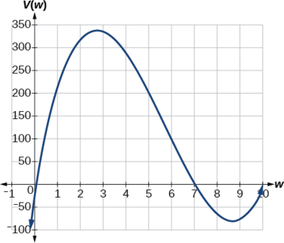
Graph of V(w)=(20-2w)(14-2w)w where the x-axis is labeled w and the y-axis is labeled V(w). — Figure $\PageIndex{24}$: Graph of $Five(westward)=(20-2w)(14-2w)w$

From this graph, we turn our focus to only the portion on the reasonable domain, $[0, 7]$. We tin estimate the maximum value to exist around 340 cubic cm, which occurs when the squares are about 2.75 cm on each side. To improve this gauge, we could use avant-garde features of our applied science, if available, or simply alter our window to zoom in on our graph to produce Figure $\PageIndex{25}$.

Graph of V(w)=(20-2w)(14-2w)w where the x-axis is labeled w and the y-axis is labeled V(w) on the domain [2.4, 3]. — Figure $\PageIndex{25}$: Graph of $V(due west)=(twenty-2w)(14-2w)w$.

From this zoomed-in view, we can refine our estimate for the maximum volume to about 339 cubic cm, when the squares measure approximately 2.seven cm on each side.

Exercise $\PageIndex{one}$

Use technology to find the maximum and minimum values on the interval $[−1,four]$ of the function $f(10)=−0.2(x−2)^3(10+i)^two(10−4)$.

Answer: The minimum occurs at approximately the point $(0,−6.five)$,
and the maximum occurs at approximately the betoken $(iii.five,7)$.

Key Concepts

Polynomial functions of degree 2 or more are smooth, continuous functions.
To find the zeros of a polynomial function, if it can be factored, factor the function and fix each factor equal to zero.
Another way to discover the 10-intercepts of a polynomial function is to graph the function and identify the points at which the graph crosses the x-centrality.
The multiplicity of a zero determines how the graph behaves at the ten-intercepts.
The graph of a polynomial will cross the horizontal centrality at a cypher with odd multiplicity.
The graph of a polynomial will bear upon the horizontal centrality at a cypher with even multiplicity.
The end behavior of a polynomial function depends on the leading term.
The graph of a polynomial function changes direction at its turning points.
A polynomial function of degree $due north$ has at about $northward−1$ turning points.
To graph polynomial functions, find the zeros and their multiplicities, determine the end behavior, and ensure that the final graph has at most $n−one$ turning points.
Graphing a polynomial part helps to estimate local and global extremas.
The Intermediate Value Theorem tells us that if $f(a)$ and $f(b)$ have reverse signs, so there exists at least one value $c$ between $a$ and $b$ for which $f(c)=0$.

Glossary

global maximum
highest turning indicate on a graph; $f(a)$ where $f(a){\geq}f(x)$ for all $x$.

global minimum
everyman turning point on a graph; $f(a)$ where $f(a){\leq}f(x)$ for all $10$.

Intermediate Value Theorem
for two numbers $a$ and $b$ in the domain of $f$, if $a<b$ and $f(a){\neq}f(b)$, and so the functionf takes on every value between $f(a)$ and $f(b)$; specifically, when a polynomial role changes from a negative value to a positive value, the role must cross the 10-axis

multiplicity
the number of times a given gene appears in the factored form of the equation of a polynomial; if a polynomial contains a factor of the grade $(x−h)^p$, $ten=h$ is a null of multiplicity $p$.